分支定界闭环检测的原理和实现
在一些SLAM系统中,通过闭环检测让机器人意识到它曾经到过某个场景,进而可以通过一些优化手段进一步的调整地图,提高定位和建图的精度。在Cartographer中, 我们可以把计算路径节点与子图之间的INTER_SUBMAP类型的约束看做是闭环检测。在上一篇文章中, 我们分析了对象constraint_builder_是如何在后台组织这一计算过程的。而算法核心则是由类FastCorrelativeScanMatcher2D提供。
本文中,我们先研究一下论文,了解分支定界的闭环检测算法原理, 再详细分析类FastCorrelativeScanMatcher2D了解其具体实现。
1. 算法原理
在Local SLAM中,通过在子图中的Scan-to-map匹配过程可以得到了一个比较理想的机器人位姿估计。 但由于Local SLAM只使用了一段时间内的局部信息,所以定位误差还会随着时间累积。为了能够进一步的降低局部误差累积的影响,Cartographer还需要通过Pixel-accurate扫描匹配来进行闭环检测, 进一步的优化机器人的位姿估计。
记\(H = \{h_1, \cdots, h_k, \cdots, h_K\}\)为传感器扫描到的\(K\)个hit点集合,\(h_k\)是第\(k\)个hit点在机器人坐标系下的位置坐标。 那么\(h_k\)在地图坐标系下的坐标可以表示为:
$$ \begin{equation}\label{f1} T_{\varepsilon} h_k = \begin{bmatrix} \cos \varepsilon_{\theta} & - \sin \varepsilon_{\theta} \\ \sin \varepsilon_{\theta} & \cos \varepsilon_{\theta} \end{bmatrix}h_k + \begin{bmatrix} \varepsilon_x \\ \varepsilon_y \end{bmatrix} \end{equation} $$其中,\(\varepsilon = \begin{bmatrix} \varepsilon_x & \varepsilon_y & \varepsilon_{\theta} \end{bmatrix}^T\)表示位姿估计\(\varepsilon_x, \varepsilon_y\)分别是机器人在地图坐标系下的坐标, \(\varepsilon_{\theta}\)是机器人的方向角。用\(T_{\varepsilon}\)表示位姿估计描述的坐标变换。那么Pixel-accurate扫描匹配问题可以用下式来描述:
$$ \begin{equation}\label{f2}\begin{split} \varepsilon^* = \underset{\varepsilon \in \mathcal{W}}{\text{argmax}} \sum_{k = 1}^K M_{nearest}\left(T_{\varepsilon}h_k\right) \end{split} \end{equation} $$上式中,\(\mathcal{W}\)是一个搜索窗口,\(M_{nearest}\left(T_{\varepsilon}h_k\right)\)是离\(T_{\varepsilon}h_k\)最近的栅格单元的占用概率。上式可以解释为, 在搜索窗口\(\mathcal{W}\)中找到一个最优的位姿,使得hit点集合出现的概率最大化。 原文中给出了一个暴力的搜索方法,如右图所示,这是一种枚举的方法。 给定搜索步长\(r\)和\(\delta_{\theta}\),该搜索过程以\(\varepsilon_0\)为中心,通过三层循环遍历所有的Pixel并选出得分最高的位姿作为输出\(\varepsilon^*\)。
显然如果搜索窗口过大或者搜索步长太小,都将导致整个搜索过程耗时过长。为了提高算法的效率,Cartographer选择使用分支定界的方法来搜索位姿。该算法的基本思想就是, 把整个解空间用一棵树来表示,其根节点代表整个搜索窗口\(\mathcal{W}\)。树中的每一个节点的孩子都是对该节点所代表的搜索空间的一个划分,每个叶子节点都对应着一个解。
整个搜索过程的基本思想,就是不断地分割搜索空间,这个过程称为分支。为每次分支之后的孩子节点确定一个上界,这个过程称为定界。 如果一个节点的定界超出了已知最优解的值,这意味着该节点下的所有解都不可能比已知解更优,将不再分支该节点。这样很多分支就不会继续搜索了,可以缩小搜索范围,提高算法效率。
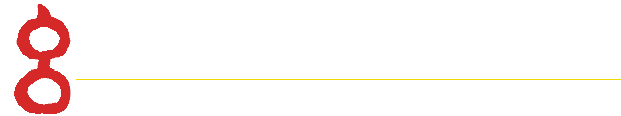
Cartographer使用一种深度优先(Depth-First Search, DFS)的搜索方法,其算法的流程如左图所示。该算法设定了一个阈值score_threshold,约定了解的下界,如果一个节点的上界比它还小, 说明这个解空间实在太烂了,就不用考虑它了。
整个搜索过程借助了一个栈\(\{\mathcal{C}\}\)来完成,首先将整个搜索空间\(\mathcal{W}\)分割,得到初始的子空间节点集合\(\{\mathcal{C_0}\}\)。 然后对集合\(\{\mathcal{C_0}\}\)中的节点根据它们的上界进行排序,并依次入栈\(\{\mathcal{C}\}\)保证得分最高的节点在栈顶的位置。这样可以优先搜索最有可能的解空间。
只要栈\(\{\mathcal{C}\}\)不空,就需要进行深度优先搜索。首先从栈顶中出栈一个搜索节点\(c\),如果\(c\)的上界比当前最优解的值高,则进一步的对该节点分割,否则认为该节点不具竞争力抛弃之。 如果该节点就是一个叶子节点,就更新最优解。否则进行分支得到新的搜索节点集合\(\{\mathcal{C_c}\}\),并为该集合中的节点定界。仍然根据节点的上界对集合\(\{\mathcal{C_c}\}\)进行排序, 并将之压入栈中,保证\(\{\mathcal{C_c}\}\)中最优的节点在栈顶的位置。
这种深度优先的搜索方法,能够尽可能的得到一个更优的解,使得best_score得到较快的增长。这样就可以达到压缩搜索空间的目的。显然该算法的实现关键在于分支和定界方法。
我们知道在二维空间中,机器人的位姿实际上是由\(x,y,\theta\)三个量来表示的。 那么搜索窗口的栅格索引集合\(\overline{\mathcal{W}}\)可以通过笛卡尔积\(\{-w_x, \cdots, w_x\} \times \{-w_y, \cdots, w_y\} \times \{-w_{\theta}, \cdots, w_{\theta}\}\)来枚举。 其中\(w_x, w_y\)分别是\(x\)和\(y\)方向上最大的搜索索引,\(w_{\theta}\)则是搜索角度的最大索引。 那么搜索窗口\(\mathcal{W}\)就可以用集合\(\left\{\varepsilon_0 + (r j_x, r j_y, \delta_{\theta} j_{\theta})\ \big|\ (j_x, j_y, j_{\theta}) \in \overline{\mathcal{W}} \right\}\)来表示, 其中,\(\varepsilon_0\)是搜索中心,也是机器人位姿的初始估计。\(r\)和\(\delta_{\theta}\)分别是位移和角度的搜索步长。
搜索树中的每个节点都可以用四个整数\(c = \left(c_x, c_y, c_{\theta}, c_h\right) \in \mathbb{Z}^4\)来表示,其中\(c_x,c_y\)分别是其搜索空间所对应的\(x,y\)轴的起始索引, \(c_{\theta}\)是搜索角度,\(c_h\)则说明了该搜索空间下一共有\(2^{c_h} \times 2^{c_h}\)个可能的解,它们具有相同的搜索角度,但位置坐标不同。 这些解的组合方式可以用如下的笛卡尔积来表示:
$$ \overline{\mathcal{U_c}} = \left\{\left(j_x, j_y\right) \in \mathbb{Z^2}\ \bigg|\ \begin{array}{} c_x ≤ j_x < c_x + 2^{c_h} \\ c_y ≤ j_y < c_y + 2^{c_h} \end{array}\right\} \times \{c_{\theta}\}$$
该节点所对应的搜索空间的栅格索引集合为\(\overline{W_c} = \overline{\mathcal{U_c}} \cap \overline{\mathcal{W}}\)。对于叶子节点而言, \(c_h = 0\),其搜索空间中只有一个索引对应着解\(\varepsilon_c = \varepsilon_0 + \left(rc_x, rc_y, \delta_{\theta}c_{\theta} \right)\)。 每当对节点进行分支,就相当于在空间坐标上将搜索空间划分为四个区域,如右图所示。如果我们指定了搜索树的高度\(h_0\),那么初始的子空间节点集合中的节点\(c \in \{C_0\}\)的四个整数可以表示为:
$$ c = \begin{cases} c_x & = & -w_x + 2^{h_0}j_x & : j_x \in \mathbb{Z}, 0 ≤ 2^{h_0} j_x ≤ 2w_x \\ c_y & = & -w_y + 2^{h_0}j_y & : j_y \in \mathbb{Z}, 0 ≤ 2^{h_0} j_y ≤ 2w_y \\ c_{\theta} & = & j_{\theta} & : j_{\theta} \in \mathbb{Z}, -w_{\theta} ≤ j_{\theta} ≤ w_{\theta}\\ c_h & = & h_0 \\ \end{cases} $$搜索树上的每个节点的上界可以通过下式计算得到:
$$ \begin{array}{rcl}\begin{split} score(c) & = & \sum_{k = 1}^K \underset{j \in \overline{\mathcal{U_c}}}{\max} M_{nearest}\left(T_{\varepsilon_j}, h_k \right) \\ & ≥ & \sum_{k = 1}^K \underset{j \in \overline{\mathcal{W_c}}}{\max} M_{nearest}\left(T_{\varepsilon_j}, h_k \right) \\ & ≥ & \underset{j \in \overline{\mathcal{W_c}}}{\max} \sum_{k = 1}^K M_{nearest}\left(T_{\varepsilon_j}, h_k \right) \end{split}\end{array} $$如果我们对于每个节点都直接通过下式计算一遍上界的话,将是一个很大的计算量。所以Cartographer仍然采取了一种空间换时间的方法来进一步的提高搜索效率。它采用一种类似图像金字塔的方法, 预先计算出占用栅格地图在不同分枝尺寸下的上界,在实际计算上界时只需要根据\(c_h\)查询对应尺度下的占用栅格即可获得节点的上界。 下图是从原文中抠出来的分枝尺寸分别为1、4、16、64时的占用概率上界。
 |
| 图 1: 分枝尺寸分别为1、4、16、64时的占用概率上界 |
我们就暂时称这个图为预算图吧,那么对于第\(h\)层的节点,在预算图中\(x,y\)的占用上界可以表示成下式,即以考察点\(x,y\)为起点, 尺寸为\(2^h \times 2^h\)的窗口内栅格的最高占用概率作为上界。
$$ \begin{equation}\label{f3} M_{precomp}^h (x, y) = \underset{\begin{array}{} x' \in \left[x, x + r(2^h -1)\right] \\ y' \in \left[y, y + r(2^h - 1) \right] \end{array}}{max}M_{nearest}(x', y') \end{equation} $$那么节点\(c\)的上界就可以直接查表得到:
$$ \begin{split} score(c) = \sum_{k = 1}^K M_{precomp}^{c_h} (T_{\varepsilon}h_k) \end{split} $$所以,我们可以认为整个闭环检测的业务逻辑就是,根据当前的子图构建一个占用栅格地图,然后为该地图计算预算图,接着通过深度优先的分枝定界搜索算法估计机器人的位姿, 最后建立机器人位姿与子图之间的约束关系。 下面我们来详细了解一下这个分支定界搜索的实现细节。
        struct SubmapScanMatcher {
            const Grid2D* grid;
            std::unique_ptr<scan_matching::FastCorrelativeScanMatcher2D>
                            fast_correlative_scan_matcher;
            std::weak_ptr<common::Task> creation_task_handle;
        };
2. FastCorrelativeScanMatcher2D
在分析约束构建器的时候, 我们就已经看到对象constraint_builder_为每个子图都构建了一个SubmapScanMatcher类型的扫描匹配器。这个扫描匹配器是定义在类ConstraintBuilder2D内部的一个结构体。 如右侧的代码片段所示,它有三个字段,分别记录子图的占用栅格、扫描匹配器内核、线程池任务句柄。
实际上闭环检测是由类FastCorrelativeScanMatcher2D完成的。下表中列出了该类的成员变量。
| 对象名称 | 对象类型 | 说明 |
|---|---|---|
| options_ | FastCorrelativeScanMatcherOptions2D | 关于闭环检测的扫描匹配器的各种配置 |
| limits_ | MapLimits | 子图的地图作用范围,我们已经在分析占用栅格的数据结构的时候, 简单了解了该数据结构的字段和作用。 |
| precomputation_grid_stack_ | PrecomputationGridStack2D | 预算图的存储结构,用于查询不同分支尺寸下的搜索节点上界。 |
下面是类FastCorrelativeScanMatcher2D的构造函数,它有两个输入参数,其中grid是子图的占用栅格,options则记录了各种配置项。 在它的成员构造列表中,完成了三个成员的构造。
        FastCorrelativeScanMatcher2D::FastCorrelativeScanMatcher2D(const Grid2D& grid,
                                                                   const proto::FastCorrelativeScanMatcherOptions2D& options)
            : options_(options),
              limits_(grid.limits()),
              precomputation_grid_stack_(common::make_unique<PrecomputationGridStack2D>(grid, options)) {}
我们已经看到该类使用了一个PrecomputationGridStack2D的数据类型来存储预算图。实际上它只是一个容器而已,只有一个成员变量precomputation_grids_。 实际的预算图是在PrecomputationGrid2D对象构建的时候计算的。由于预算图的计算过程没有耍什么花样,所以我们不详细分析了。
std::vector<PrecomputationGrid2D> precomputation_grids_;
在上文中, 我们了解到约束构建器通过变量match_full_submap来选择全地图匹配或者是定点的局部匹配。下面是定点局部匹配的接口函数,它有5个输入参数, 其中initial_pose_estimate描述了初始的位姿估计;point_cloud则是将要考察的路径节点下的激光点云数据;min_score是一个搜索节点的最小得分, 也就是前文中提到的score_threshold;指针score和pose_estimate是两个输出参数,用于成功匹配后返回匹配度和位姿估计。
        bool FastCorrelativeScanMatcher2D::Match(const transform::Rigid2d& initial_pose_estimate,
                                                 const sensor::PointCloud& point_cloud,
                                                 const float min_score, float* score,
                                                 transform::Rigid2d* pose_estimate) const {
            const SearchParameters search_parameters(options_.linear_search_window(),
                                                     options_.angular_search_window(),
                                                     point_cloud, limits_.resolution());
            return MatchWithSearchParameters(search_parameters, initial_pose_estimate, point_cloud, min_score, score, pose_estimate);
        }
上面代码的第5到7行,构建了一个SearchParameters类型的对象,这是一个定义在correlative_scan_matcher_2d.h中的一个结构体,它描述了搜索窗口以及分辨率。然后在第8行中通过调用函数MatchWithSearchParameters来实际完成扫描匹配,进而实现闭环检测。
下面的代码是用于全地图匹配的接口函数,它的只是少了描述初始位姿的输入参数,其他参数的意义都与刚刚的定点局部匹配是一样的。殊途同归, 全地图匹配也是调用函数MatchWithSearchParameters来实际完成扫描匹配的。所不同的是,它需要提供一个以子图中心为搜索起点,覆盖整个子图的搜索窗口。 所以我们会看到第3到7行构建的对象search_parameters和center。
        bool FastCorrelativeScanMatcher2D::MatchFullSubmap(const sensor::PointCloud& point_cloud, float min_score, float* score,
                                                           transform::Rigid2d* pose_estimate) const {
            const SearchParameters search_parameters(1e6 * limits_.resolution(),  // Linear search window, 1e6 cells/direction.
                                                     M_PI,  // Angular search window, 180 degrees in both directions.
                                                     point_cloud, limits_.resolution());
            const transform::Rigid2d center = transform::Rigid2d::Translation(limits_.max() - 0.5 * limits_.resolution() *
                                              Eigen::Vector2d(limits_.cell_limits().num_y_cells, limits_.cell_limits().num_x_cells));
            return MatchWithSearchParameters(search_parameters, center, point_cloud, min_score, score, pose_estimate);
        }
3. 分支定界搜索
接下来我们就从这个MatchWithSearchParameters函数出发研究这个深度优先的分支定界搜索算法,下面是这个函数的代码片段,它有6个输入参数,只是比定点局部匹配的接口函数多了一个search_parameters的参数, 其他参数的意义都一样。search_parameters描述了窗口大小、分辨率等搜索信息。在函数的一开始先检查一下指针score和pose_estimate非空,因为在后续的计算过程中将要修改这两个指针所指对象的数据内容。
        bool FastCorrelativeScanMatcher2D::MatchWithSearchParameters(SearchParameters search_parameters,
                                                                     const transform::Rigid2d& initial_pose_estimate,
                                                                     const sensor::PointCloud& point_cloud,
                                                                     float min_score, float* score,
                                                                     transform::Rigid2d* pose_estimate) const {
            CHECK_NOTNULL(score);
            CHECK_NOTNULL(pose_estimate);
然后,获取初始位姿估计的方向角,将激光点云中的点都绕Z轴转动相应的角度得到rotated_point_cloud。
            const Eigen::Rotation2Dd initial_rotation = initial_pose_estimate.rotation();
            const sensor::PointCloud rotated_point_cloud = sensor::TransformPointCloud(point_cloud,
                transform::Rigid3f::Rotation(Eigen::AngleAxisf(initial_rotation.cast<float>().angle(), Eigen::Vector3f::UnitZ())));
调用定义在correlative_scan_matcher_2d.cc中的函数GenerateRotatedScans获得搜索窗口下机器人朝向各个方向角时的点云数据。 也就是说容器rotated_scans中保存了姿态为\(\varepsilon_0 + (0, 0, \delta_{\theta}j_{\theta}), j_{\theta} \in \mathbb{Z}, -w_{\theta} ≤ j_{\theta} ≤ w_{\theta}\)时所有的点云数据, 其中\(\varepsilon_0\)就是这里的初始位姿估计initial_pose_estimate,\(\delta_{\theta}\)则是角度搜索步长,它由对象search_parameters描述。
const std::vector<sensor::PointCloud> rotated_scans = GenerateRotatedScans(rotated_point_cloud, search_parameters);
接着通过同样定义在correlative_scan_matcher_2d.cc中的函数DiscretizeScans,
完成对旋转后的点云数据离散化的操作,即将浮点类型的点云数据转换成整型的栅格单元索引。
类型DiscreteScan2D就是通过typedef std::vector<Eigen::Array2i> DiscreteScan2D;定义的整型容器。
在接下来的第14行中,我们通过对象search_parameters的接口ShrinkToFit尽可能的缩小搜索窗口的大小,以减小搜索空间,提高搜索效率。
            const std::vector<DiscreteScan2D> discrete_scans = DiscretizeScans(limits_, rotated_scans,
                            Eigen::Translation2f(initial_pose_estimate.translation().x(), initial_pose_estimate.translation().y()));
            search_parameters.ShrinkToFit(discrete_scans, limits_.cell_limits());
准备工作做完之后,下面就要进入实际的搜索过程了。首先通过函数ComputeLowestResolutionCandidates完成对搜索空间的第一次分割,得到初始子空间节点集合\(\{C_0\}\)。 该函数在最低分辨率的栅格地图上查表得到各个搜索节点\(c \in \{C_0\}\)的上界,并降序排列。
            const std::vector<Candidate2D> lowest_resolution_candidates =
                ComputeLowestResolutionCandidates(discrete_scans, search_parameters);
最后调用函数BranchAndBound完成分支定界搜索,搜索的结果将被保存在best_candidate中。检查最优解的值,如果大于指定阈值min_score就认为匹配成功, 修改输入参数指针score和pose_estimate所指的对象。否则认为不匹配,不存在闭环,直接返回。
            const Candidate2D best_candidate = BranchAndBound(discrete_scans, search_parameters, lowest_resolution_candidates, precomputation_grid_stack_->max_depth(), min_score);
            if (best_candidate.score > min_score) {
                *score = best_candidate.score;
                *pose_estimate = transform::Rigid2d({initial_pose_estimate.translation().x() + best_candidate.x, initial_pose_estimate.translation().y() + best_candidate.y}, initial_rotation * Eigen::Rotation2Dd(best_candidate.orientation));
                return true;
            }
            return false;
        }
在研究ComputeLowestResolutionCandidates和BranchAndBound的实现之前,先来看一下数据类型Candidate2D, 它是定义在correlative_scan_matcher_2d.h中的一个结构体。下表中列举了该结构体的成员变量。
| 对象名称 | 对象类型 | 说明 |
|---|---|---|
| scan_index | int | 角度的搜索索引\(j_{\theta}\) |
| x_index_offset | int | x轴的搜索索引\(j_{x}\) |
| y_index_offset | int | y轴的搜索索引\(j_{y}\) |
| x | double | 相对于初始位姿的x偏移量\(rj_x\) |
| y | double | 相对于初始位姿的y偏移量\(rj_y\) |
| orientation | double | 相对于初始位姿的角度偏移量\(\delta_{\theta}j_{\theta}\) |
| score | float | 候选点的评分,越高越好 |
此外,它还定义了两个比较操作符的重载用于方便比较候选点的优劣。
        bool operator<(const Candidate2D& other) const { return score < other.score; }
        bool operator>(const Candidate2D& other) const { return score > other.score; }
下面是函数ComputeLowestResolutionCandidates的实现,它以离散化之后的各搜索方向上的点云数据和搜索配置为输入,先调用函数GenerateLowestResolutionCandidates完成对搜索空间的初始分割, 再通过函数ScoreCandidates计算各个候选点的评分并排序。
        std::vector<Candidate2D> FastCorrelativeScanMatcher2D::ComputeLowestResolutionCandidates(
                                    const std::vector<DiscreteScan2D>& discrete_scans,
                                    const SearchParameters& search_parameters) const {
            std::vector<Candidate2D> lowest_resolution_candidates = GenerateLowestResolutionCandidates(search_parameters);
            ScoreCandidates(precomputation_grid_stack_->Get(precomputation_grid_stack_->max_depth()),
                            discrete_scans, search_parameters, &lowest_resolution_candidates);
            return lowest_resolution_candidates;
        }
下面是函数GenerateLowestResolutionCandidates的代码片段,它根据搜索配置来完成初始分割。首先根据预算图的金字塔高度计算初始分割的粒度\(2^{h_0}\)。
        std::vector<Candidate2D>
        FastCorrelativeScanMatcher2D::GenerateLowestResolutionCandidates(const SearchParameters& search_parameters) const {
            const int linear_step_size = 1 << precomputation_grid_stack_->max_depth();
然后遍历所有搜索方向,累计各个方向下空间的分割数量,得到num_candidates描述了搜索空间初始分割的子空间数量。
            int num_candidates = 0;
            for (int scan_index = 0; scan_index != search_parameters.num_scans; ++scan_index) {
                const int num_lowest_resolution_linear_x_candidates = (search_parameters.linear_bounds[scan_index].max_x -
                                  search_parameters.linear_bounds[scan_index].min_x + linear_step_size) / linear_step_size;
                const int num_lowest_resolution_linear_y_candidates = (search_parameters.linear_bounds[scan_index].max_y -
                                  search_parameters.linear_bounds[scan_index].min_y + linear_step_size) / linear_step_size;
                num_candidates += num_lowest_resolution_linear_x_candidates * num_lowest_resolution_linear_y_candidates;
            }
接下来在一个三层的嵌套for循环中,构建各个候选点。最后检查一下候选点数量,通过后返回。
            std::vector<Candidate2D> candidates;
            candidates.reserve(num_candidates);
            for (int scan_index = 0; scan_index != search_parameters.num_scans; ++scan_index) {
            for (int x_index_offset = search_parameters.linear_bounds[scan_index].min_x;
                 x_index_offset <= search_parameters.linear_bounds[scan_index].max_x;
                 x_index_offset += linear_step_size) {
            for (int y_index_offset = search_parameters.linear_bounds[scan_index].min_y;
                 y_index_offset <= search_parameters.linear_bounds[scan_index].max_y;
                 y_index_offset += linear_step_size) {
                candidates.emplace_back(scan_index, x_index_offset, y_index_offset, search_parameters);
            } } }
            CHECK_EQ(candidates.size(), num_candidates);
            return candidates;
        }
下面是函数ScoreCandidates的实现,该函数有四个参数,其中precomputation_grid是将要查询的预算图,而discrete_scans则是离散化的各搜索角度下的激光点云,而search_parameters则是搜索配置, candidates则是候选点集合将在本函数中计算得分并排序。在函数中,我们在一个for循环中遍历所有的候选点,并为之计算所有点云的hit概率。最后通过std::sort完成排序。
        void FastCorrelativeScanMatcher2D::ScoreCandidates(const PrecomputationGrid2D& precomputation_grid,
                                                           const std::vector<DiscreteScan2D>& discrete_scans,
                                                           const SearchParameters& search_parameters,
                                                           std::vector<Candidate2D>* const candidates) const {
            for (Candidate2D& candidate : *candidates) {
                int sum = 0;
                for (const Eigen::Array2i& xy_index : discrete_scans[candidate.scan_index]) {
                    const Eigen::Array2i proposed_xy_index(xy_index.x() + candidate.x_index_offset, xy_index.y() + candidate.y_index_offset);
                    sum += precomputation_grid.GetValue(proposed_xy_index);
                }
                candidate.score = precomputation_grid.ToScore(sum / static_cast(discrete_scans[candidate.scan_index].size()));
            }
            std::sort(candidates->begin(), candidates->end(), std::greater());
        }
下面是函数BranchAndBound,具体完成了分支定界搜索过程,输入参数就不一一介绍了,参考后面的注释。
        Candidate2D FastCorrelativeScanMatcher2D::BranchAndBound(const std::vector<DiscreteScan2D>& discrete_scans, // 离散化的各搜索角度下的激光点云
                                                                 const SearchParameters& search_parameters,        // 搜索配置参数
                                                                 const std::vector<Candidate2D>& candidates,       // 候选点集
                                                                 const int candidate_depth,                        // 搜索树高度,前文提到的c_h
                                                                 float min_score) const {                          // 候选点最小评分
这个函数是以递归调用的方式求解的。首先给出了递归终止的条件,就是如果搜索树高为0,意味着我们搜索到了一个叶子节点。同时由于每次迭代过程我们都是对新扩展的候选点进行降序排列, 所以可以认为队首的这个叶子节点就是我们想要的最优解,直接返回即可。
            if (candidate_depth == 0)
                return *candidates.begin();
然后创建一个临时的候选点对象best_high_resolution_candidate,为之赋予最小的评分。
            Candidate2D best_high_resolution_candidate(0, 0, 0, search_parameters);
            best_high_resolution_candidate.score = min_score;
接着就会在一个for循环中遍历所有的候选点,如果遇到一个候选点的评分很低,意味着以后的候选点中也没有合适的解。可以直接跳出循环退出了,说明没有构成闭环。
            for (const Candidate2D& candidate : candidates) {
                if (candidate.score <= min_score)
                    break;
如果for循环能够继续运行,说明当前候选点是一个更优的选择,需要对其进行分支。新生成的候选点将被保存在容器higher_resolution_candidates中。
                std::vector<Candidate2D> higher_resolution_candidates;
                const int half_width = 1 << (candidate_depth - 1);
                for (int x_offset : {0, half_width}) {
                    if (candidate.x_index_offset + x_offset > search_parameters.linear_bounds[candidate.scan_index].max_x)
                        break;
                    for (int y_offset : {0, half_width}) {
                        if (candidate.y_index_offset + y_offset > search_parameters.linear_bounds[candidate.scan_index].max_y) {
                            break;
                    }
                    higher_resolution_candidates.emplace_back(candidate.scan_index, candidate.x_index_offset + x_offset, candidate.y_index_offset + y_offset, search_parameters);
                }
            }
再然后就调用刚刚介绍过的函数ScoreCandidates对新扩展的候选点定界并排序。并递归调用BranchAndBound对新扩展的higher_resolution_candidates进行搜索。 这样就可以实现深度优先的搜索,先一直沿着最有可能的分支向下搜索,直到找到一个解。并将该解作为目前的最优解保存在best_high_resolution_candidate中。 以后通过递归调用发现了更优的解都将通过std::max函数来更新已知的最优解。
            ScoreCandidates(precomputation_grid_stack_->Get(candidate_depth - 1), discrete_scans, search_parameters, &higher_resolution_candidates);
            best_high_resolution_candidate = std::max(best_high_resolution_candidate,
                                                      BranchAndBound(discrete_scans, search_parameters, higher_resolution_candidates, candidate_depth - 1,
                                                                     best_high_resolution_candidate.score));
当遍历完所有的候选点之后,对象best_high_resolution_candidate中就记录了最优的解,将之返回即可。
            }
            return best_high_resolution_candidate;
        }
至此,我们已经看到了完整的分支定界搜索过程。
4. 完
Cartographer使用类FastCorrelativeScanMatcher2D具体实现了,深度优先的分支定界搜索算法,该算法能够高效地确定激光点云与子图的匹配度,估计采集点云时机器人相对于子图的位姿。 为了能够高效的对搜索空间进行分割并计算上界,Cartographer还为每个子图预先计算了不同尺度下的占用概率,以后的搜索过程只需要简单的查表就可以完成了。